Randomness makes parallelization interesting

A friend of mine recently posed a problem which seems at first blush quite simple but turns out to be quite interesting. Suppose you have a program which takes $T$ time and which is perfectly parallelizable — that is, I can split the program up into $K$ tasks and the latency for the program will be $T / K$ .
So I can make the latency arbitrarily small by taking $K \rightarrow \infty$ .

So why wouldn’t you ever just set $K$ as large as conceivably possible? Well, suppose there were a fixed startup cost associated with each task, $S$ . Then, the latency would be $S + T/K$ . Again, it’s clear that you should just parallelize the hell out of your program and eventually your latency will approach $S$ .

But what if the startup cost were random? Let the startup cost be drawn from some probability distribution $S_i \sim f$ . Now each subtask will take a different amount of time; since I’m concerned with the latency, the metric I want to optimize is $\max_{i\in \{1\ldots K\}} S_i + T/K$ over $K$ .

Now there’s a cool tradeoff involved in parallelization: one the one hand, splitting a task reduces the $T/K$ part of the equation, but on the other, it increases the number of draws of $S_i$ and therefore the expected maximum value.

It turns out that the solution to this problem leads down a huge rabbit hole involving order statistics, sample maxima, and extreme value statistics. Here are some highlights:

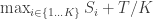
The probability distribution of the maximum value in a sample of $K$ draws from a distribution $f$ is given by $K F(x)^{K-1} f(x)$ where $F$ is the cumulative distribution function (There’s a more general form for the $i$ th order statistic).
The expected value of the maximum (drawn according to the procedure above) is $\int_{0}^1 F^{-1}(x^{1/K}) dx$ , where $F^{-1}$ is the inverse cdf (or quantile) function. For almost all distributions this expression cannot be computed analytically (The uniform distribution being the notable exception).
When $f = \mathrm{Unif}(a, b)$ , the analytical solution to the expected maximum value is $a + (b - a) \frac{K}{K+1}$ . This leads to a quadratic polynomial as the solution of the original problem. Without loss of generality, let $b-a = 1$ . Then the optimal value of $K$ takes the form $\frac{T + \sqrt{T}}{1-T}$ . Note that when $T > 1$ the roots are negative, i.e., one should set $K$ to infinity. The interesting range is between 0 and 1. I’ve attached a plot of this function for this range here. You’ll notice that the bend is quiet steep so that you’ll want the parallelization to either be very small or very large depending on how long your program takes relative to the startup costs.
When $f$ is not uniform, things are more difficult. I’m not entirely sure what the right model is for the costs, but I think and exponential distribution might make a first cut. Using a numerical approximation, I computed latencies as a function of $K$ for various values of $T$ and rate parameter set to 1 here (the values of $T$ are in the title of each plot). Because of the long tails, one needs to be much more cautious before parallelizing. For values of $T$ explored here you generally shouldn’t to go above $K = 5$ . Also, the different performance for different values of $K$ can be quite substantial, but bang/buck is questionable. For example, when $T=5$ if you spend 5 times as many resources, you’ll go almost twice as fast. Is that a worthwhile investment? When $T=1$ you almost definitely don’t want to parallelize at all.

Ok, so it seemed like a simple little problem at first, but it turns out that something as straightforward sounding as parallelization can lead to some pretty interesting analysis.

5 responses to “Randomness makes parallelization interesting”

Indraneel

March 13, 2009 at 1:01 pm

Another application of the result you just mentioned( min(X1,..,Xk) is concentrated around 1/k when Xi are (pairwise?) independently drawn from the uniform distribution) is finding the number of distinct elements in a massive stream of data of size m consisting of elements from a massive set {1,…,n}, where you are only allowed O(log m + log n) storage.

- Kevin Nuckolls
  
  April 24, 2009 at 2:06 am
  
  I am interested in knowing how to perform this type of analysis. I have a math minor focused more on graph theory and linear algebra. Can you point me to some good statistics resources for this kind of thing?
  
  - Indraneel
    
    April 28, 2009 at 3:10 am
    
    You can find the proofs in a paper at
    
    http://portal.acm.org/citation.cfm?id=237823
    
    Some of the math used can be found in the following great book:
    
    The Probabilistic Method – Noga Alon and Joel Spencer
    
    You could take a look at relevant chapters a text on randomized algorithm (a standard is “Randomized Algorithms” by Motwani and Raghawan). These are more discrete math and algorithms rather than statistics references, but they contain everything you need to understand the proofs in the paper.
J Kujala

May 1, 2009 at 2:02 pm

You assume that you start only a single task of each type. If startup costs are independent for several copies of the same task, then it makes sense to start a very large number of instances of the same task.

- slycoder
  
  May 5, 2009 at 9:01 pm
  
  You’re totally right; if we replicate each task we can take the min, that is $\max_{i \in \{1\ldots K\}} \min_{j \in \{1 \ldots R\}} S_{ij} + T / K$ . Then it clearly makes sense to make $R$ as large as possible. Although, in cases when you also want to make $K$ as large as possible, I wonder what you want $R / K$ to be, that is, how you should divide resources between tasks and task replicates.