
I once heard it on good authority that Gelman says you usually don’t need more than 12 samples. Well, as a result of a discussion with Sam Gershman (sorry Sam for not answering the actual question you asked!), I wondered if that was true; that is, if under reasonable assumptions it might be better to take a small number of samples. Caveat: there’s probably lots of work on this already, but where would the fun be in that?
Ok, let’s assume that your goal is to estimate ![\mathbb{E}_{z \sim p(z | x)}[f(z)]](https://s0.wp.com/latex.php?latex=%5Cmathbb%7BE%7D_%7Bz+%5Csim+p%28z+%7C+x%29%7D%5Bf%28z%29%5D&bg=ffffff&fg=333333&s=0&c=20201002)


- that your sampler has mixed and that you’re getting independent samples (that condition alone should give you fair warning that what I’m about to say is of little practical value);
- to obtain
samples from the sampler costs some amount, say
.
More samples are usually better, because they’ll give you a better representation of the true distribution, i.e. ![\mathbb{E}_{z \sim \hat{p_n}(z | x)}[f(z)] \rightarrow \mathbb{E}_{z \sim p(z | x)}[f(z)]](https://s0.wp.com/latex.php?latex=%5Cmathbb%7BE%7D_%7Bz+%5Csim+%5Chat%7Bp_n%7D%28z+%7C+x%29%7D%5Bf%28z%29%5D+%5Crightarrow+%5Cmathbb%7BE%7D_%7Bz+%5Csim+p%28z+%7C+x%29%7D%5Bf%28z%29%5D&bg=ffffff&fg=333333&s=0&c=20201002)

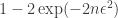
We can define a loss by ![\ell = R(n) + |\mathbb{E}_{z \sim \hat{p_n}(z | x)}[f(z)] - \mathbb{E}_{z \sim p(z | x)}[f(z)]|](https://s0.wp.com/latex.php?latex=%5Cell+%3D+R%28n%29+%2B+%7C%5Cmathbb%7BE%7D_%7Bz+%5Csim+%5Chat%7Bp_n%7D%28z+%7C+x%29%7D%5Bf%28z%29%5D+-+%5Cmathbb%7BE%7D_%7Bz+%5Csim+p%28z+%7C+x%29%7D%5Bf%28z%29%5D%7C&bg=ffffff&fg=333333&s=0&c=20201002)

If your cost is linear, 
something like 


The plot below shows what might happen if you make such a choice. Here, I've let the posterior be an equiprobable binomial distribution. The function I'm computing is the identity 


Turns out for some reasonable values, you really should stick to about 12 samples.


Pingback: The cost of a sample « visualization, etc.
I like the accuracy vs. time dimension. It fits in with Monsieur Gelman’s continual blog comments about sticking to justified significant digits. Especially when you look at some of his hierarchical models that have very few items from which to estimate means.
This reminds me, for some reason, of the SGD vs. quasi-Newton methods like L-BFGS for fitting regression models. SGD’s way faster at getting to a couple significant digits, but slower for getting to lots of significant digits.
Yeah, a lot of statisticians love lots of significant digits which is odd since they should be the first to recognize that many of those digits are useless.
As for SGD vs. L-BFGS, in my experience both SGD and L-BFGS are terrible for getting to lots of significant digits =).