
I once heard it on good authority that Gelman says you usually don’t need more than 12 samples. Well, as a result of a discussion with Sam Gershman (sorry Sam for not answering the actual question you asked!), I wondered if that was true; that is, if under reasonable assumptions it might be better to take a small number of samples. Caveat: there’s probably lots of work on this already, but where would the fun be in that?
Ok, let’s assume that your goal is to estimate ![\mathbb{E}_{z \sim p(z | x)}[f(z)]](https://s0.wp.com/latex.php?latex=%5Cmathbb%7BE%7D_%7Bz+%5Csim+p%28z+%7C+x%29%7D%5Bf%28z%29%5D&bg=ffffff&fg=333333&s=0&c=20201002)


- that your sampler has mixed and that you’re getting independent samples (that condition alone should give you fair warning that what I’m about to say is of little practical value);
- to obtain
samples from the sampler costs some amount, say
.
More samples are usually better, because they’ll give you a better representation of the true distribution, i.e. ![\mathbb{E}_{z \sim \hat{p_n}(z | x)}[f(z)] \rightarrow \mathbb{E}_{z \sim p(z | x)}[f(z)]](https://s0.wp.com/latex.php?latex=%5Cmathbb%7BE%7D_%7Bz+%5Csim+%5Chat%7Bp_n%7D%28z+%7C+x%29%7D%5Bf%28z%29%5D+%5Crightarrow+%5Cmathbb%7BE%7D_%7Bz+%5Csim+p%28z+%7C+x%29%7D%5Bf%28z%29%5D&bg=ffffff&fg=333333&s=0&c=20201002)

We can define a loss by ![\ell = R(n) + |\mathbb{E}_{z \sim \hat{p_n}(z | x)}[f(z)] - \mathbb{E}_{z \sim p(z | x)}[f(z)]|](https://s0.wp.com/latex.php?latex=%5Cell+%3D+R%28n%29+%2B+%7C%5Cmathbb%7BE%7D_%7Bz+%5Csim+%5Chat%7Bp_n%7D%28z+%7C+x%29%7D%5Bf%28z%29%5D+-+%5Cmathbb%7BE%7D_%7Bz+%5Csim+p%28z+%7C+x%29%7D%5Bf%28z%29%5D%7C&bg=ffffff&fg=333333&s=0&c=20201002)

If your cost is linear, 
something like 


The plot below shows what might happen if you make such a choice. Here, I've let the posterior be an equiprobable binomial distribution. The function I'm computing is the identity 


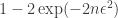
Turns out for some reasonable values, you really should stick to about 12 samples.

