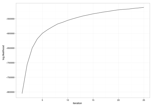
Dave gently reminded me that properly assessing convergence of our models is important and that just running a sampler for N iterations is unsatisfactory. I agree wholeheartedly. As a first step, the collapsed Gibbs sampler in the R LDA package can now optionally report the log likelihood (to within a constant). For example, we can rerun the model fit in demo(lda) but with an extra flag set:
result <- lda.collapsed.gibbs.sampler(cora.documents,
                                      K,  ## Num clusters
                                      cora.vocab,
                                      25,  ## Num iterations
                                      0.1,
                                      0.1,
                                      compute.log.likelihood=TRUE)
Using the now-available variable result$log.likelihoods, we can plot the progress of the sampler versus iteration:
Grab it while it’s hot: http://www.cs.princeton.edu/~jcone/lda_1.0.1.tar.gz.


I agree with Dave! I finally took Martin Jansche’s advice and refactored LingPipe’s Java implementation of collapsed Gibbs for LDA to return an iterator over Gibbs samples. (The original implementation, which is still there, took a callback function to apply to each sample.)
One thing the sample lets you do is compute the corpus log likelihood given the parameters. Note that this is just the likelihood, not the prior. Did you include the Dirichlet prior or just p(docs|topics)? And did you sum over all possible topic assignments, or just evaluate the probability of the actual one?
I do the same thing, only with the coefficient prior as well, for the SGD implementation of logistic regression.
Hi,
I also wanted to do an iterator approach but laziness overtook me =).
As for what I compute, it’s the joint likelihood given a sample of topic assignments .
.
Could you please explain a little more in regards to how you calculate the log-likelihood? I’ll tell you what I understand:
To make things clear, let’s say we have: (K – # of topics, M – # of documents, V – # of unique terms)
ndsum[j] = total # of words in document j, size M
nwsum[i] = total # of words assigned to topic i, size K
and
nw[i][j] = # of words i assigned to topic j
nd[i][j] = # of words in doc i assigned to topic j
Now, for each m document, you sum all the log-gamma(nds + alpha) and subtract the ndsums. Then for each k topics, you sum all the log-gamma(nws + beta) and subtract the nwsums.
Is this the technique that you use for log-likelihood evaluation? Does this correspond to evaluating log(P(z = j | all other z, w, d, alpha, beta))? I’m referring to this paper: http://psiexp.ss.uci.edu/research/papers/SteyversGriffithsLSABookFormatted.pdf
Best regards,
Adnan
You are more or less correct – that is how I’m computing log likelihood (see line 832 of gibbs.c in the package for details). I should point out that it is not the conditional probability of a single assignment but rather the joint probability over a set of assignments: log p(z_1, z_2, z_3, … | w, alpha, beta). It gets computed after an entire gibbs sweep over the variables.
how to plot log-likelihood vs iteration in R LDA
I’d recommend asking on the topic-models mailing list as there are many practitioners there who can help you.